Main research interests

In a very short time, language models have gone from producing mathematical results that simply seemed plausible to solving olympiad problems and now to providing proofs of open research questions. The discipline is booming: websites listing open problems, such as the Erdős problem database, now contain dozens of machine-generated proposals, many of which are likely correct, but for which no human expert has volunteered to vouch for them, and in several cases, the human author of the proposal has even declared himself unqualified to do so.
During his public lecture at the most recent International Congress of Mathematicians, Tao focused his talk on the impact of this situation on the profession, which he described as a crisis in the foundations of mathematical values and practices [136]. His assessment is that mathematical research pursues several objectives at once: solving problems, developing theories, understanding, and training the next generation. These elements have always been positively correlated, so that progress made in one could serve as an indicator for the others, and most of them could remain implicit. Thurston already summed it up in 1994: we are not trying to meet some abstract quota of definitions, theorems, and proofs, and the measure of success lies in the fact that we do enables people to understand and think more clearly [133]. A proof is the starting point of understanding, not its end result. A tool that produces correct proofs without enabling understanding breaks the equilibrium. As a consequence, the usual indicators no longer reflect what they once represented and they must therefore be replaced. This replacement has already begun to take institutional form. The Leiden Declaration on Artificial Intelligence and Mathematics, published in June 2026 [139], states precisely what had not been said before: that a proof must not only confer certainty on its conclusion, but also enable an understanding of why that conclusion is true, and that merit and responsibility continue to lie with humans. It calls for the disclosure of automated tools and for authors to remain responsible for the accuracy of every argument and every citation; it does not call for the prohibition of any element.
With regard to this redefinition of proof, which is viewed more as an explanation than as a guarantee of certainty, I find the concept of cognitive debt particularly interesting. This term is borrowed from the concept of technical debt in software engineering, a metaphor used by Cunningham to refer to the future cost of a shortcut taken today [128]. In its current sense, this term was coined by Willshire in 2025 to describe the situation in which one forgoes critical thinking for the sole purpose of obtaining answers, without truly understanding why those answers are what they are [129], and it became widely used thanks to an experiment on essay writing conducted at the MIT Media Lab [130]. Precisely, cognitive debt is the invisible, accumulated liability incurred when one obtains a result without the understanding that would normally have produced it. Performance seems satisfactory as long as the tool is present; the deficit only becomes apparent when the scaffolding is removed.
It should be noted that, in mathematics, incurring such a debt is not a problem. In fact, it naturally follows from citing a theorem as a black box without having understood all the details of its proof. In a way, that is what a theorem is for. In particular, we know that mathematical knowledge can accumulate faster than cognitive debt can be repaid, as illustrated by the example of the classification of finite simple groups: approximately 20,000 pages of journal articles, about 500 papers, around 100 authors, announced in 1983, and not a single living person who understands the argument in its entirety. Gorenstein, who had the best overview of the situation, had warned that if the techniques were forgotten before the proof was presented in an accessible form, the theorem “would gradually disappear from the living world of mathematics, buried deep within the dusty pages of forgotten journals”; he died in 1992 [134]. From the perspective of cognitive debt, the second-generation proof by Gorenstein, Lyons, and Solomon [135], which is still in progress, is nothing else than a repayment project.
With current language models, this phenomenon can even occur at the individual level. Indeed, to take full advantage of a language model when tackling a mathematical problem, one must ask well-formulated questions and let the agent work on them through numerous iterations, rather than simply chatting with it. The results are long, verbose files containing proofs whose level of detail is not suited for a human reader and which, in addition, may contain errors. That is when the debt begins. The agent identifies a difficulty and proposes an approach; we tell it to go ahead; a few iterations later, we no longer understand the difficulty, the approach, or why the approach was supposed to solve it. Nothing seems to have gone wrong. We’ve simply ceased to be the person capable of understanding.
To continue the metaphor, the questions to ask ourselves now are: What is the interest rate, and is there a repayment plan? No one can restructure our understanding for us, so we’ll have to do it ourselves. What I suggest is converting such an unreadable LLM-generated file into a digest: a ten-to-fifteen-page document from which we can judge whether the arguments are clear and correct, without opening the source draft. It’s intended to be run at a specific moment; namely, as soon as we notice that the agent is attempting something that can no longer be justified by ourselves. This avoids routine checks and keeps the logical structure at the surface, so that the state of the draft becomes visible in an afternoon rather than over two weeks. I wrote it as a skill for Claude Code; that is, a file that reconfigures the agent for a single task, and the examples and development history are publicly available.
I used and developed this Claude skill and methodology while working on the preprint [102]. After several sessions with the LLM, I ended up with a 70-page draft on Alexandrov geometry and optimal transport, on which the agent had gotten stuck, unable to make any further progress despite several results already having been established. I couldn’t figure out where the bug was hiding in all those 70 highly detailed pages. Talking with the agent didn't help me understand the problem any better. After running the skill, I received a sixteen-page summary that allowed me to spot the hidden error, which was elementary: a proof by contradiction in which the negated statement was incorrectly negated. That single error was what had caused the agent to get stuck in a loop of increasingly complex and dead-end reasoning. Note that the digest did not detect the error, nor does it contain anything that would allow one to search for one; it made the argument readable, and I did the rest: I paid off my debt.
Let me point out some of the limitations of this skill. First, its output, the digest, is a readable draft and not a publishable paper. Second, it was calibrated using a single article on metric geometry, which does not call into question the rules regarding style or logical structure, but rather what the tool considers routine and therefore removes. Any contributions are welcome to help test it and extend its use to other areas of mathematics.

A Riemannian structure is the specification of a means of measuring lengths. From a practical point of view, this can be considered as the choice of a system of units of measurement, but the mathematical abstraction goes a little further and allows this system of measurements to depend on where the measurement is actually taken. Of all those possible systems, the one we are familiar with, and in which the Pythagorean theorem we learned at school is valid, is called ‘Euclidean’, named after the Greek mathematician Euclid.
Given a smooth space with a Riemannian structure, the Riemann curvature tensor is a mathematical object that measures how far the local geometry deviates from Euclidean geometry. It is null if, and only if, the space is Euclidean, and moreover, it completely characterises the geometry, in the sense that, given the Riemann curvature tensor, we can completely recover the Riemannian metric structure. From a physical point of view, the Riemann curvature tensor at a point in space describes the tidal forces that would affect a physical body located at that point.
By considering only the average effect of Riemann curvature, which mathematically consists of contracting the tensor, we obtain the Ricci curvature tensor, which has become a central concept since the formulation of general relativity, and in particular Einstein's revolutionary statement that the Ricci tensor of spacetime is equal to the energy-momentum tensor \(\textbf{T}\) compensated by half of its trace \(T\) times the metric \(g\), up to Newton's universal constant \(G\), hence asserting that spacetime is deformed by the matter it contains: \[ \mathrm{Ric} = 8\pi G \left( \textbf{T} - \frac{1}{2} T g\right). \]
The property for a space to have a Ricci tensor bounded below by some \(K\in\mathbb{R}\) therefore means in some sense that this space contains at least an amount \(K\) of energy, and has many implications, including the Bishop-Gromov inequality for the growth of the volume of its geodesic balls, the local Poincaré inequality, the local doubling condition, the Cheeger-Gromoll splitting theorem, Myers's theorem for its diameter, or the Lichnerowicz inequality for its fundamental frequency.
Moreover, given some \(K\in\mathbb{R}\) and some \(N\in\mathbb{N}\), the class \(R_{K,N}\) of all Riemannian manifolds of dimension \(n\leq N\) having a Ricci tensor bounded below by \(K\), form a totally bounded space for the Gromov-Hausdorff topology. The theory of so-called Ricci-limit spaces, appearing from limit of sequence of manifolds in \(R_{K,N}\), has been developped in the nineties by Cheeger and Colding, see e.g. [1].
Since the Gromov-Hausdorff topology does not assume the type of smoothness of the manifold structure, the search for the closure of \(R_{K,N}\) is in some way equivalent to the search for a synthetic notion of curvature bounded below, that is a notion that does not involve any differential manifold structure.
To date, we do not yet have a synthetic notion of lower bounded Ricci curvature that corresponds exactly to the closure of \(R_{K,N}\) with respect to the Gromov-Hausdorff topology. However, there are several very interesting synthetic notions, all of which correspond to a class strictly larger than the closure of \(R_{K,N}\).
The class of spaces \(\mathrm{CD}(K,N)\) is certainly the most important historically. It was defined using optimal transport by Sturm [87,88] and Lott and Villani [77], as spaces with a geodesically convex entropy functional on the Wasserstein space \(W_2\), which is the space of probability distributions with finite second moments, equipped with the \(L^2\)-optimal transport distance. Note that the letters \(\mathrm{CD}\) stand for ‘curvature-dimension’.
A more refined version is the class of \(\mathrm{RCD}(K,N)\) spaces, which were defined by Ambrosio-Gigli-Savaré [37] as \(CD(K,N)\) spaces having a quadratic Cheeger energy, a property known as infinitesimal Hilbertianity and ensuring that tangent spaces are Euclidean by asking the Sobolev space \(W^{1,2}\) to be a Hilbert space. Note that here the letter \(R\) stands for Riemann.
Today, the class \(\mathrm{RCD}(K,N)\) seems to be the best way to look at the closure of \(R_{K,N}\), even if both are not equal, see [67], and this is due to the large amount of research successfully done to show that the good properties of manifolds in \(R_{K,N}\) are still true for \(\mathrm{RCD}\) spaces. In particular, the Bishop-Gromov inequality and all theorems listed above remain true for \(\mathrm{RCD}(K,N)\) spaces. My contribution [45] with Brunel and Ohta is part of this objective, generalizing Grünbaum's inequality, which is a classical result in the Minkowski theory of convex sets, to the setting of \(\mathrm{RCD}(0,N)\) spaces.
Several studies in this field have yielded results that were even new in the smooth case. For example, Lichnerowicz's quantitative inequality in the case of essentially non-branching \(\mathrm{CD}(K,N)\) spaces by Cavalletti, Mondino and Semola [61], and its strengthening in the case of \(\mathrm{RCD}\) spaces in my collaboration with Fathi and Gentil [64].
For a very nice exposition on the topic of spaces with curvature bounded below, we refer the reader to Tewodrose's PhD thesis [91]. Let us mention some other very interesting synthetic notion for Ricci curvature bounded below, including the Measure-Contraction property introduced by Ohta [66], defined in terms of the contraction of a measure on a set to a point; the Bishop-Gromov synthetic Ricci curvature introduced by Besson and Gallot [65], defined in terms of the growth of the volume of balls; or the barycenter curvature-dimension condition introduced by Han, Liu and Zhu in [69], in terms of Wasserstein barycenters.

From the point of view of \(\mathrm{RCD}\) spaces, the notions of space and volume are formalized in the axiomatic of metric measure spaces. It is possible to understand those notions in a rather different manner by mean of Brownian motions. For more intuition about it, see my thesis manuscript [82]. The idea is not to understand a space in itself, but to understand a space through a stochastic motion within that space, usually named Brownian motion for historical reasons. There are two main rigorous formalizations of this intuition that are possible: one using Bakry-Émery theory, the other using the concept of Dirichlet forms.
The formalization by means of the Bakry-Émery theory is in fact equivalent to the description of \(\mathrm{RCD}\) spaces given above, up to the technical assumption known as the Sobolev-to-Lipschitz property, see [68]. For a brief introduction to the Bakry-Émery theory, see the section Dynamical \(\Gamma\)-calculus.
Formalization using Dirichlet spaces consists of starting from a notion of energy, called Dirichlet energy, and considering stochastic motion as a particle following the (random) trajectory that minimises this energy, see [71]. This formalization makes it possible, in particular, to study singular spaces such as fractals, see for example [38]. Dirichlet and \(\mathrm{RCD}\) spaces are closely related. This is actually proved by Suzuki's deep result [90] stating that under the \(\mathrm{RCD}\) condition, the pointed measure Gromov convergence is equivalent to the weak convergence of Brownian motions.

General relativity was the main starting point for the development of Ricci curvature theory, so it is natural to want to adapt the synthetic notion of curvature bounded below to the case of Lorentzian spaces, that is spacetime geometry. We refer the reader to Cavalletti and Mondino [60] for a review of this theory.

At the heart of the theory described in the previous section lies a single equivalence: the Ricci curvature is nonnegative if and only if the Boltzmann entropy is convex along the \(W_2-\)geodesics. Unlike the Ricci tensor, whose definition requires regularity, the \(W_2-\)convexity of the entropy does not require it, which therefore allows to define a synthetic notion of a Ricci lower bound on non-smooth metric spaces. A natural question that arises is whether this procedure can be extended to the lower bound of sectional curvature. Since the Ricci curvature is the trace of the curvature tensor, a natural hypothesis would be to find a matrix such that its trace is equal to the entropy. One might therefore expect that the displacement convexity of such a matrix would carry the sectional curvature. Such a matrix entropy has been intrduced by Shenfeld [94] and then Aishwarya, Rotem and Shenfeld [93].
Let us describe it. For \(\mu_0,\mu_1\) two compactly supported probability measures with a density, let \(\theta\) be the Kantorovich potential between them for the quadratic cost. Let \((\theta_t)_{t>0}\) be its Hamilton-Jacobi flow, defined by \(\partial_s\theta_s +\tfrac12 |\nabla\theta_s|^2 =0\), and whose characteristics are the transport rays \(\gamma_x(s) = \exp_x(s\nabla\theta(x))\). Along such a ray set \[ U_s := \mathrm{Hess}\,\theta_s \qquad \quad \mathrm{and} \qquad \quad E_t := -\int_0^t U_s\, ds. \] The matrix \(E_t\) is the entropy tensor, satisfying the identity \(H(\mu_t) = H(\mu_0) + \int \mathrm{Tr}\,E_t\, d\mu_0\), with \(H\) denoting the Boltzmann entropy. One says that \(E\) is matrix displacement convex, abbreviated (MDC), if \begin{equation}\label{MDC} \ddot E_t \succeq \left( \dot E_t \right)^2 \quad \text{in the Loewner order,} \qquad \text{equivalently} \qquad \dot U_t \preceq - U_t^2 . \end{equation} Since on Euclidean space the Hessians of the interpolating potentials solve the flat Riccati equation \(\dot U = -U^2\), the condition says that the Hessian flow along the ray is dominated by the flat Riccati flow issued from the same initial condition. The \((\mathrm{MDC})\) condition is therefore a comparison condition.
On a manifold, \(U\) solves \(\dot U_s + U_s^2 + R_s = 0\) with \(R_s\) given by \(\langle R_s w,w\rangle = \mathrm{Sec}(\dot\gamma,w)|\dot\gamma|^2\), for all \(w\perp\dot\gamma\) with unit norm. So \eqref{MDC} holds along a ray exactly when the planes tangent to the transport have nonnegative sectional curvature. Aishwarya, Rotem and Shenfeld concluded that \((\mathrm{MDC})\) for all pairs of measures, characterises \(\mathrm{Sec}\geq 0\). Note that taking traces recovers the Lott-Villani-Sturm equivalence for \(\mathrm{Ric}\geq 0\).
To complete the program, we must show that the equivalence holds even in the absence of a smooth structure. Since sectional curvature already has a synthetic notion of a lower bound, namely, Alexandrov’s geometry [2], which defines it by comparing geodesic triangles with their Euclidean counterparts, the task is then to show that the condition \((\mathrm{MDC})\) is equivalent to non-negative curvature in the Alexandrov sense. Note that the scalar part of the problem had already been solved by Petrunin [96]: a finite-dimensional Alexandrov space with \(\mathrm{curv}\geq 0\) satisfies the entropy convexity condition \(\mathrm{CD}(0,N)\).
In [102], I showed that the equivalence \((\mathrm{MDC}) \Leftrightarrow \mathrm{curv}\ge 0\) also holds in the Alexandrov setting. The main difficulty lay in the fact that, in order to give meaning to the condition \((\mathrm{MDC})\) itself, it was necessary to resort to the notion of synthetic parallel transport so that \(E_t\) would be well-defined. Furthermore, this parallel transport must satisfy certain properties, such as the cocycle property, which ensures that the integral defining the entropy matrix does not depend on the identification path used to construct it, and the second variation bound, which allows us to obtain \eqref{MDC} from the definition of the Hamilton-Jacobi flow. Each synthetic parallel transport proposed in the literature satisfies one of these properties but not the other: Petrunin’s parallel transport [95] satisfies the second-variation bound but not the cocycle property; and the connection obtained from the \(C^0\)-Riemannian structure of Otsu and Shioya [97] yields the cocycle identity, but its Christoffel symbols are only Radon measure, for which no second-variation formula is available. One of the main results of [102] is to refine Petrunin's construction to get a synthetic parallel transport having both properties.
Note that, when defined along the rays of a transport, the condition \((\mathrm{MDC})\) is Lagrangian. Since a finite-dimensional Alexandrov space is, in particular, an \(\mathrm{RCD}\) space, Gigli’s second-order calculation [98] applies to it and yields a distributive Riemannian curvature tensor [99], which gives it a second Eulerian interpretation: one tests the Riccati inequality with respect to a fixed vector field rather than a parallel frame. The last result in [102] is that the non-negative Gigli sectional curvature corresponds exactly to the Eulerian form of the \((\mathrm{MDC})\) property. The question of whether the Lagrangian and Eulerian interpretations are equivalent remains open and boils down to comparing the different synthetic notions of parallel transport: Petrunin’s and the one formalized on \(\mathrm{RCD}\) spaces by Gigli and Pasqualetto [100,101]. An affirmative answer would allow to establish Gigli’s conjecture, according to which the lower bounds of the sectional curvature of his tensor characterize the Alexandrov condition among \(\mathrm{RCD}\) spaces.

Although traditionally seen as rather distinct areas of mathematics, statistics and geometry have, in recent years, developed a rapidly growing interface, with many insights to be gained on both sides. At a high level, geometry enters statistics through the structure of the data.
It is clear that certain types of data naturally possess a geometric structure. A typical example arises in shape analysis, whose aim is to automatically detect similarities between the shapes of objects in a database, with applications such as face recognition. However, the striking feature of recent decades is that geometric data structures appear almost universally, because they are related to the internal correlations in the data, which is almost always the case for high-dimensional data.
Statistical estimation has long been confronted with the challenge of high dimensionality. When data points \(X_1, \dots, X_N\) lie in a space \(\mathbb{R}^D\) with \(D \gg 1\), a situation that frequently occurs in practice today, for instance when the \(X_i\) are audiovisual files with ambient dimension on the order of several millions, statistical estimation rapidly becomes computationally demanding. This difficulty is commonly known as the curse of dimensionality, a term introduced by Bellman in his 1957 book [12], where he explicitly emphasized how the explosive growth of volume in high-dimensional spaces renders data increasingly sparse and isolated.
To illustrate how our low-dimensional intuitions (in dimensions 2 or 3) can fail in higher dimensions, let us mention Stein’s celebrated paper [6], in which he showed that in dimensions greater than three, the usual estimator of the mean is no longer optimal in terms of quadratic risk. This phenomenon is now known as Stein’s paradox.
When working with high-dimensional data, it is often unrealistic to assume that the data are truly generated by a process with as many degrees of freedom as the ambient dimension. Consider, for example, photographs of hands. Such images are naturally embedded in a Euclidean space whose dimension equals the number of pixels. However, it would be unreasonable to believe that a hand can vary freely in so many directions. In reality, the effective degrees of freedom are much closer to the number of joints in the hand, at most a few dozens, which is dramatically smaller than the number of pixels (on the order of \(5\) million).
Therefore, when dealing with high-dimensional data, the most natural way to model randomness is not through a uniform measure, as in lower-dimensional settings, but rather through a probability distribution supported on a lower-dimensional manifold. In this framework, the data \((X_1,\dots,X_n)\) are assumed to lie on a submanifold \(\mathcal{M}\subset \mathbb{R}^D\). This perspective on high-dimensional data is now widely known as the manifold hypothesis, and it continues to be an active area of research in statistics. To mention just a few contributions: Belkin and Niyogi’s 2009 conference [9], the work of Fefferman et al.~[8], which develops statistical tests to assess the validity of the manifold hypothesis; and, on a more playful note, the paper [11] showing that \(3\times 3\) image patches naturally form a Klein bottle.
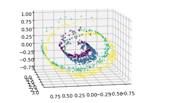
My personal view on the variety hypothesis is that, instead of considering a random variable as a measurable mapping from a probability space, \(X : (\Omega,\,\mathbb{P}) \to (\mathbb{R}^D,\mu)\), we consider it as a mapping between metric measure spaces, \(X : (\Omega, \mathrm{dist}, \mathbb{P}) \to (\mathcal{M}, d_{\mathcal{M}}, \mu)\). In addition to the classical statistical task of estimating the distribution \(\mu\), this new perspective also requires estimating \(d_{\mathcal{M}}\) from the sample, a process known as metric learning.

Of course, real data are inevitably affected by noise, so the model suggested by the manifold hypothesis is more accurately described as "manifold + noise". From this viewpoint, several fundamental questions naturally arise, among which the three most prominent are:

• Metric learning, which consists in identifying the manifold \(\mathcal{M}\) itself,
• Clustering, which focuses on detecting the connected (or nearly connected) components of \(\mathcal{M}\),
• Dimensionality reduction, which seeks to embed the manifold \(\mathcal{M}\) into a lower-dimensional space of dimension \(d\ll D\), \(\mathcal{M}\subset \mathcal{N}^d \subset \mathbb{R}^D\).

Let us expand a little further on the notion of dimensionality reduction. Linear techniques such as Principal Component Analysis (PCA) are well-established and widely used, but they suffer from a crucial drawback: they fail to capture the intrinsic structure of the data. This limitation becomes particularly problematic when working with highly structured data. In response, recent years have witnessed the development of nonlinear dimensionality-reduction methods, which essentially project the data onto a lower dimensional submanifold \(\mathcal{N}^d \subset \mathbb{R}^D\). From this perspective, the problem of metric learning can be viewed as the most refined form of dimensionality reduction, since it amounts to recovering the manifold \(\mathcal{M}\) itself. However, \(\mathcal{M}\) cannot always be accurately approximated, and in practice it is often sufficient to identify another manifold \(\mathcal{N}^d \subset \mathbb{R}^D\), as long as \(d \ll D\). A wide variety of techniques have been proposed in this direction, notably Laplacian eigenmaps [15], ISOMAP [16], and diffusion maps [17], to mention just a few. Let us also highlight the role of autoencoders [7], a class of neural networks specifically designed to learn a representation of data in a latent space, which can be interpreted as a compressed encoding of the original data while preserving its most relevant features.
In the area of deep learning, a particularly exciting connection between statistics and geometry arises through the attention mechanism of transformers. Roughly speaking, the procedure begins by dividing a text into small blocks, called tokens, which are then represented in a high-dimensional space so that tokens with similar usage in the text are mapped to nearby points. This representation is known as word embedding, and can be adapted to data types beyond text. The attention mechanism, or more precisely the self-attention mechanism [10], then analyzes the importance of each token relative to all the others in the embedding space. In this way, the meaning assigned to each token is determined by its context, and is therefore inherently contextual.
Put in more intuitive terms, large language models demonstrate that the meaning of words can effectively be reduced to a geometry of words, and the self-attention mechanism provides a means of computing this geometry.\\
Another way to view the interplay between geometry and statistics is to observe that when certain information on a manifold is learnable, i.e., can be efficiently approximated by statistical estimators, this reflects less a property of the estimators themselves than a statistical property of the underlying geometry. From this perspective, the most universal results seems to be Gromov’s reconstruction theorem, which states that a metric measure space is uniquely determined by the law of the distance matrix between samples of arbitrary size [13]. See also [14] for a proof based on the law of large numbers. More specific geometric properties also give rise to statistical consequences, and two of them organise the sections that follow: upper bounds on the sectional curvature lead to finite-sample bounds for barycenters, while non-negative lower bounds on the Ricci curvature translate into notions of statistical depth.

Let us expand a little on upper bounds for sectional curvature. Just as lower bounds on Ricci curvature can be characterized in a synthetic way, that is, without any reference to differentiability (see the section Spaces with Ricci curvature bounded below), upper (and likewise lower) bounds on sectional curvature can also be described synthetically by means of triangle comparison. This leads to what is known as Alexandrov geometry [2]. The key idea is based on Toponogov’s theorem, which states that if a Riemannian manifold has sectional curvature everywhere bounded above by some \(\kappa \in \mathbb{R}\), then its geodesic triangles are thinner than the corresponding triangles in the model space of constant curvature \(\kappa\): hyperbolic space if \(\kappa < 0\), Euclidean space if \(\kappa = 0\), and the sphere if \(\kappa > 0\). Since the notion of a triangle makes sense even in the non-smooth setting of a geodesic metric space, Alexandrov curvature provides a way to define curvature bounds directly through triangle comparison. In particular, an upper bound on sectional curvature implies a local strong geodesic convexity of the squared distance to any point. In the case of nonpositive sectional curvature, this geodesic convexity is even global. Such convexity properties provide a natural framework to define and study the notion of a mean or barycenter. The most celebrated, and perhaps the most intuitive, statistical estimator in Euclidean space is the empirical mean, given by \[ S_n = \frac{1}{n} \sum_{i=1}^n X_i \] for an i.i.d data set \((X_1, \dots, X_n) \in (\mathbb{R}^d)^n\). One of the simplest properties of \(S_n\) is its linearity in the data points \(X_i\). However, when the data lie in a non-linear space, \((X_1, \dots, X_n) \in \mathcal{M}^n\), the usual linear definition of the mean no longer applies. A natural way to generalize \(S_n\) to a non-linear setting is to observe that it is the least squares estimator, that is, \begin{equation}\label{leastsquare} S_n \in \underset{p \in \mathcal{M}}{\mathrm{argmin}} \frac{1}{n} \sum_{i=1}^n d(p,X_i)^2 \end{equation} Minimizing this quantity makes sense in any metric space, and the resulting points are known as Fréchet means [3]. The Fréchet mean enjoys properties of uniqueness, consistency and asymptotic normality, which are closely related to upper bounds on the sectional curvature of the space through the geodesic convexity properties mentioned above, see [46,47]. An iterative procedure to approximate the minimizer of Problem \eqref{leastsquare} can be performed via a stochastic gradient-type descent, as introduced by Sturm [89]. In the case of nonpositive sectional curvature, the resulting inductive mean \(b_n\) converges to the population barycenter \(b^*\), and in particular, \[ \mathbb{E} \left[ d(b^*, b_n)^2 \right] \leq \frac{\sigma^2}{n}, \] where \(\sigma^2 = \mathbb{E} \left[ d(b^*, X_1)^2 \right]\) is the variance. Moreover, this convergence can be strengthened into a Bernstein-type concentration bound: for all \(\delta \in (0,1)\), it holds with probability at least \(1-\delta\) that \[ d(b^*, b_n) \leq \frac{\sigma}{\sqrt{n}} + K \sqrt{\frac{\log(1/\delta)}{n}}, \] when \(X_1\) is \(K^2\)-sub-Gaussian, see my contribution with Brunel [49]. From the perspective of the correspondence between statistics and geometry, our results show that in a space that is less curved than Euclidean space, the means exhibit statistical properties that are at least as good as those in the Euclidean model.
See [48] for the case of a positive sectional curvature upper bound (\(\kappa > 0\)), where the analysis is more involved and the bounds are not yet sharp. These results are also obtained in collaboration with Brunel.

The barycenter discussed in the previous section summarizes a data set as a single point, which is meaningful only when the data form a single cluster. When the data form multiple groups, the natural object of interest is a small family of points, each summarizing a cluster, rather than a single point. A very popular estimator that produces this is the \(K\)-means method. Let \(X\) be a random variable taking values in a metric space \((M,d)\). The population and empirical \(K\)-means are given by \[ \underset{\#A \leq k}{\mathrm{argmin}}\ \mathbb{E}\left[ \min_{a\in A} d(X,a)^2 \right], \qquad \qquad \underset{\#A \leq k}{\mathrm{argmin}}\ \frac{1}{n}\sum_{i=1}^n \min_{a \in A} d(X_i,a)^2, \] the minimisation running over subsets \(A\) of at most \(k\) points, called centroids. Each centroid is associated with its Voronoi cell, that is, the set of points closer to it than to any other centroid. These cells are called clusters. Setting \(k=1\) yields exactly the Fréchet mean from the previous section. 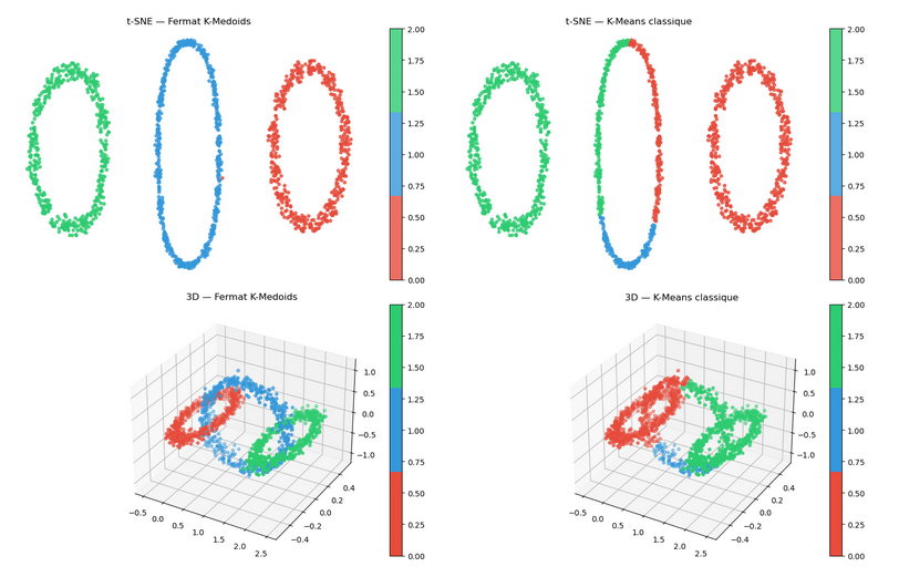At the other extreme, when \(k\) is large, this same minimization corresponds to the problem of quantization of a measure, that is, finding the best approximation of \(\mu\) by a measure defined on at most \(k\) points [113]; the interest then lies in \(k \gg 1\) and in the speed with which the approximation improves, rather than in the separation of the groups.

In the Euclidean setting, the algorithmic and theoretical framework is standard. Lloyd’s algorithm [118] alternates between assigning each point to its nearest centroid and moving each centroid toward the mean of its cell, and Pollard [110] proved that, when the solution of the \(K\)-means method is unique, the empirical solution converges to it almost surely. Uniqueness constitutes a significant restriction, and Lember [111] studied what remains without this restriction; more recently, Jaffe [112] developed an asymptotic theory covering the geometric framework and the adaptive choice of \(k\).
Under the manifold hypothesis, the data are regarded as mappings between metric measure spaces, \(X_i : (\Omega, \mathrm{dist}, \mathbb{P}) \to (\mathcal{M}, d_{\mathcal{M}}, \mu)\), and the distance \(d_{\mathcal{M}}\) is estimated from the sample, thus becoming an empirical distance. A concrete and instructive family of such estimators is built from paths through the sample itself. Let \(\mathcal{X}_n = \{x_1,\dots,x_n\} \subset \mathbb{R}^D\) and \(\alpha \geq 1\). We assign to a path \(x \to \cdots \to y\) passing through the points of the sample the length \(\sum_i \|x_{i+1}-x_i\|^\alpha\), and we let \(d_{\mathcal{X}_n,\alpha}(x,y)\) be the infimum of these paths. For \(\alpha = 1\) on a neighborhood graph, this is the ISOMAP [16]; for \(\alpha > 1\) on the complete graph, this is the Fermat distance [115]. The exponent \(\alpha\) penalizes long jumps, so that a path is “economical” when it progresses in small steps through dense regions. As a consequence, the estimator takes into account not only the shape of the support but also the density associated with it. This is formalized by a convergence theorem of Hwang, Damelin, and Hero [114] and of Groisman, Jonckheere, and Sapienza [116]: for i.i.d. data with density \(f>0\) on a sufficiently regular \(\mathcal{M}^d\), almost surely \[ n^{(\alpha-1)/d}\, d_{\mathcal{X}_n,\alpha} \underset{n\to\infty}{\longrightarrow} c_\alpha\, d_{f,\alpha}, \qquad \qquad d_{f,\alpha}(x,y) = \inf_\gamma \int_\gamma f^{(1-\alpha)/d}\, d\ell . \] The limit corresponds to the geodesic distance of a metric that is conformal with the original metric, where the conformal factor is a negative power of the density. It is therefore costly to traverse regions of low density, which corresponds exactly to the expected behavior of a distance intended to separate clusters.
An interesting problem is to obtain a consistency result in this setting, where the distance itself is estimated. In fact, the classical theory of consistency no longer applies, since Pollard’s and Lember’s theorems assume a fixed metric space. In our article [117], written in collaboration with Groisman, Jonckheere, and Sued, we addressed this gap by establishing the appropriate framework for this purpose.
Since the issue consists in establishing a joint convergence of distance and measure, the appropriate concept turns out to be the one already used by geometers: the measured Gromov–Hausdorff convergence (mGH), which requires the existence of a sequence of maps \(h_n : (\mathbb{X}_n, d_n,\mu_n) \to (\mathbb{X},d,\mu)\) that distort the distances by at most \(\varepsilon_n \to 0\) and map the measures \(\mu_n\) to measures weakly converging to \(\mu\).
Our main result in [117] is that \(K\)-means is continuous under the mGH topology. We do not assume that the population \(K\)-means is unique; therefore, we cannot expect that the empirical centroids converge to a fixed limit. What we do obtain, however, is that if the spaces \((\mathbb{X}_n, d_n,\mu_n)\) converges in the mGH topology to \((\mathbb{X},d,\mu)\), then for large \(n\), every set of empirical centroids is close to a certain set of true centroids. This is a no-false-positive guarantee. Note that when the population \(K\)-means turns out to be unique, the statement becomes the usual consistency result.
A companion result we obtained says the same thing for the clusters rather than the centroids: under the same mGH convergence assumption, for \(n\) large, each empirical Voronoi cell is contained in a slightly thickened true cell. Again, this is interpretated as a no-false-positive guarantee.
In practice, it is important to know under what conditions the mGH convergence hypothesis holds. It holds under two natural conditions that one would expect from a metric learning procedure: that the estimated distance converges uniformly to the true distance on the sample, and that the sample becomes dense in space. Since, from the Borel-Cantelli lemma, the second condition is automatically satisfied when \(\mu\) is defined on a Riemannian manifold and is absolutely continuous with respect to the volume measure, the assumption holds as long as the distance estimator is well-designed, which is in particular the case for the ISOMAP and Fermat distance estimators.

The three previous sections estimate a location: a barycenter, a family of centroids, the clusters they determine. A different but related question about a cloud of points is not where its centre is, but how central a given point is, and the answer to it is a depth.
The notion goes back to Tukey [4]. Given a probability measure \(\mu\) on \(\mathbb{R}^d\), the halfspace depth of a point \(x\) is \[ D(x) := \inf \left\{ \mu(H) \ : \ H \text{ a closed halfspace containing } x \right\}, \] that is, the smallest amount of mass one is forced to keep when cutting the space by a hyperplane. A point located near the edge of the cloud can be isolated by a half-space containing almost no mass and hence has depth close to \(0\); a point located at the center of the cloud cannot be isolated and has a large depth. Depth is therefore a way to classify data from the outside in, without ever referring to a mean or a linear structure beyond the half-spaces themselves. Points of maximum depth act as medians, and this is what makes this concept useful in practice: like the median and unlike the mean, estimators constructed from it are robust, in the sense that arbitrarily removing a small fraction of the sample does not alter them [5]. In one dimension, \(D\) is the smaller of the two tail masses, and its maximizer is exactly the median, with the value \(1/2\); in higher dimensions, the maximum depth is smaller, and by how much is a truly geometric question.
A lower bound on the maximum depth is a statement of the following form: if the mass is distributed according to a given constraint, there exists a point that is difficult to isolate. The fact that such a statement is available ultimately says more about the space in which the data are embedded than about the estimator itself.
In collaboration with Brunel and Ohta [45], we showed that, in a space with non-negative Ricci curvature, the Fréchet barycenter of a convex set is deep; where, in the definition of depth, half-spaces have been replaced by horoballs, which are the limits of geodesic balls whose centers move away toward infinity along a ray. This substitution was necessary because a general manifold does not contain Euclidean hyperplanes, and it is also the appropriate substitute, since Euclidean hyperplanes are nothing more than spheres of infinite radius whose centers are mapped to infinity.
It should be noted that this result supports our main claim: that geometric meaning becomes statistical meaning. Indeed, on the one hand, we have a purely geometric hypothesis, namely, a lower bound on the Ricci curvature; and on the other, a purely statistical conclusion, namely, the existence of a point that no horoball can easily separate from the rest of the mass, and thus the existence of a robust notion of a center of a data cloud.

A mapping \(T\) between two metric spaces is a contraction, or is \(1\)-Lipschitz, if it never increases distances. When such a mapping also transports a measure to another, it becomes a remarkably effective tool: any inequality whose two sides are governed by a gradient, which includes Poincaré, logarithmic Sobolev, and isoperimetric inequalities, as well as concentration estimates, is automatically transferred from the source space to the target space. This fact is known in the literature as the contraction principle, and it can be understood by considering that a contractive transport mapping is a weakened notion of isometry. One approach, therefore, is to prove the inequality once on a model space where the calculations are possible, and it then holds on any space that is the contractive image of that model. This is why the existence of contractive transport maps has become a topic of interest in its own right.
The founding result in this direction is Caffarelli's contraction theorem [103]. It asserts that if \(\mu = e^{-V(x)}dx\) is a probability measure on \(\mathbb{R}^n\) with \(\nabla^2 V \geq I_n\), then the Brenier optimal transport map pushing the standard Gaussian onto \(\mu\) is a contraction.
Running alongside this line of research, the following question arises. The Lichnerowicz inequality states that a compact manifold with \(\mathrm{Ric}_g \geq (n-1)g\) has a first nonzero eigenvalue greater than or equal to that of the round sphere, \(\lambda_1(g) \geq \lambda_1(g_{\mathrm{can}}) = n\), where the round sphere is the model that satisfies the equality. A natural question is whether this comparison extends to the rest of the spectrum, that is, whether \begin{equation}\label{spectralcomparison} \lambda_i(g) \geq \lambda_i(g_{\mathrm{can}}), \qquad i \geq 1, \end{equation} holds? Colding and Minicozzi highlighted this problem in 1998 as a long-standing open problem [120], motivated by Yau’s question regarding the dimension of spaces of harmonic functions with polynomial growth, for which the comparison with exact round thresholds determines the optimal Euclidean bound. The conjecture turned out to be false, and Donnelly produced a counterexample to \eqref{spectralcomparison} in dimension four and higher [121]. On the positive side, Mangasuli verified \eqref{spectralcomparison} for left-invariant metrics on \(\mathbb{S}^3\) [122], and then, on \(\mathbb{S}^2\), for any fixed \(j\) and all \(i \leq j\), for metrics obtained from the round one by an analytic, rotationally symmetric, conformal perturbation [123].
Since Donnelly's counterexample is not diffeomorphic to a sphere (it is homeomorphic to \(\mathbb{S}^2\times \mathbb{S}^2\)), it therefore did not provide an answer to the question posed regarding metrics on \(\mathbb{S}^n\) itself. And since the existence of a contractive transport map also implies the complete comparison \eqref{spectralcomparison}, Milman [105] posed the following question: if \(g\) is a metric on \(\mathbb{S}^n\) such that \(\mathrm{Ric}_g \geq (n-1)g\), does there exist a contraction \[ T : (\mathbb{S}^n, g_{\mathrm{can}}, \mathrm{vol}_{g_{\mathrm{can}}}) \longrightarrow (M^n, g, \mathrm{vol}_g) \] that maps the rescaled volume measure to \(\mathrm{vol}_g\)? Milman also formulated a family of precise conjectures, on the sphere and in the \(\mathrm{CD}(\rho,\infty)\) setting, in spectral and contraction forms.
These conjectures have since been completely resolved. Aryan constructed counterexamples on the sphere, in all dimensions \(d\geq 4\), thereby refuting the spectral and contraction conjectures [124]. The obstruction is based on a spectral mechanism: a product structure generates a high multiplicity of small eigenvalues, such that by using a clever perturbation in a certain direction of the product, \(\lambda_i\) falls below its rounded value for a certain \(i\), while the Ricci tensor remains bounded below by a positive constant. Conversely, Lin, Wang, and Xu [125] proved \eqref{spectralcomparison} for all \(i\) in dimension two, as well as a version for two-dimensional Alexandrov spheres; they also provided a counterexample to \eqref{spectralcomparison} in dimension three. Finally, Han and Zhu [126] filled the only remaining gap: by using the inverse mean curvature flow in a manner analogous to Kim and Milman’s heat flow construction, they constructed Lipschitz contractions that preserve the normalized area, thereby proving Milman’s contraction conjecture for Riemannian spheres of dimension two. In summary, Milman's conjecture is therefore true in dimension two and false in all higher dimensions. Note also that, in the case of infinite dimensions, Dudarov and Mikulincer [127], based on concentration arguments, presented a weighted manifold satisfying \(\mathrm{CD}(1/2,\infty)\) which cannot be realized as the contractive transport of a Gaussian, which thus contradicts Milman’s conjecture for in the \(\mathrm{CD}(\rho,\infty)\) setting.

My two papers on this topic prove Milman’s conjecture in a perturbative regime, that is, for manifolds close to a round sphere. At the time, they were the first positive results in its favor, and their significance lies as much in the tools they employ as in the statements themselves. Now that the conjecture has been fully resolved and we know it is false for all dimensions \(n\ge 4\), an interesting avenue of research is to find additional relevant assumptions about the metric \(g\), in addition to the positive lower bound on Ricci, such that the conjecture becomes true. From this perspective, the perturbative results represent doors left ajar.
In [108], I treated surfaces: if \(g\) is a small perturbation of a round sphere of radius strictly smaller than one, and satisfying \(\mathrm{Ric}_g \geq g\), then there exists a contraction \((\mathbb{S}^2, g_{\mathrm{can}}) \to (\mathbb{S}^2, g)\) pushing the rescaled volume measure of the unit round sphere onto \(\mathrm{vol}_g\). The proof combines three tools which we sketch now.
One starts a rescaled Ricci flow from the initial metric \(g\). On a surface this flow converges to a round sphere \(\mathbb{S}^2_\rho\) of radius \(\rho\), with \(\rho^2 = \mathrm{vol}_g(\mathbb{S}^2)/4\pi\). Now the curvature hypothesis \(\mathrm{Ric}_g\geq g\) forces \(\mathrm{vol}_g(\mathbb{S}^2) \leq 4\pi\), with equality if and only if \(g\) is exactly the unit round sphere, so that \(\rho < 1\) strictly.
Next, inspired by the Kim-Milman construction [104] for the heat flow under a fixed metric, the Ricci flow can be turned into a transport map between the volume measures of the source and target metrics. The point here is to identify the vector field driving that flow, which turns out to be the gradient of the curvature potential.
The third step is to bound the Lipschitz constant of the resulting map, which boils down to controlling the Hessian of the curvature potential. This is done through a multiscale Bakry-Émery analysis, the same family of techniques that appears in the renormalization section below, and it requires along the way a uniform version of Hamilton's theorem on the preservation of positive curvature. One is then left with a Lipschitz bound for a map whose source is \(\mathbb{S}^2_\rho\) rather than \(\mathbb{S}^2_1\), and this is where \(\rho<1\) matters: it provides just enough room for the composition with the contraction \(\mathbb{S}^2_1 \to \mathbb{S}^2_\rho\) to remain \(1\)-Lipschitz, provided the initial metric is close enough to \(\mathbb{S}^2_\rho\). Note that dimension two is used only twice, through the Gauss-Bonnet theorem and through Hamilton's theorem.
The second contribution [109], joint with Ge, removes the restriction on dimension by replacing the Kim-Milman map with the Brenier-McCann optimal transport map. The result is that every nearly spherical manifold is the volume-preserving image of a round sphere under that map: for a metric \(g\) sufficiently \(C^{0,\alpha}\)-close to the round metric of radius \(\rho\in(0,1)\), the optimal transport map for the quadratic cost of \(g_{\mathrm{can}}\), read as a map \((\mathbb{S}^n, g_{\mathrm{can}}) \to (\mathbb{S}^n, g)\), is \(1\)-Lipschitz. Since it is the optimal transport map that is shown to contract, this constitutes a perturbative extension of Caffarelli's theorem itself. Note that the unit round sphere is excluded from this result, since it is false that all small perturbations of it are contractive volume-preserving images of it.
The proof is based on a stability result for the optimal transport problem on the sphere which seems of independent interest. If two density functions \(f_1,f_2\) are sufficiently close in \(C^{0,\alpha}\)-topology, \(\alpha\in(0,1)\), then the optimal transport maps from the volume measure onto them, \(T_1: \mathrm{vol}\to f_1\mathrm{vol}\) and \(T_2:\mathrm{vol}\to f_2\mathrm{vol}\) are close in the \(C^{1,\alpha'}\)-topology, for all \(\alpha'\in(0,\alpha)\). This result is a small contribution to the growing body of literature on the stability of transport maps; see Letrouit’s course [140].

Stein's method is a set of techniques extensively developed from the seminal paper [86] of Charles Stein in 1972. The aim of these techniques is to give quantitative bound for the distance between two probability measures. This method was introduced to quantify the asymptotic normality of certain statistical estimators, and proved extremely fruitful in mathematical statistics at a time when non-asymptotic bounds were establishing themselves as major theoretical guarantees for practical applications. We refer the reader to the survey by Ross [80] which remains the most cited survey on Stein's method.
From a statistical perspective, the concept of distance between probability distributions serves as a bridge between asymptotic theory and finite sample theory. Asymptotic theory asserts that with a sufficiently large amount of data, one can accurately estimate the quantity of interest, commonly referred to as the estimand. However, "sufficient" can range from a manageable sample size to one that is practically unattainable. In contrast, finite sample theory focuses on determining the exact number of observations required to estimate the estimand with a predefined level of precision. Let us illustrate this with the example of the Central Limit Theorem (CLT). The CLT states that under mild assumptions, the empirical mean (the estimator) is asymptotically a Gaussian perturbation of the population mean (the estimand) \[ \frac{1}{n}\sum_{i=1}^n X_i \underset{n\to\infty}{\sim} \mathbb{E}[X] + \frac{1}{\sqrt{n}}\,\mathcal{N}\left(0, 1 \right). \] In this setting, distances between probability distributions are a natural concept to mathematically formalize what a level of precision is, and therefore enable us to replace the asymptotic guarantee \(\underset{n\to\infty}{\sim}\) by a quantitative bound of the form \[ \mathrm{dist}\left(\mu_n , \mathcal{N}(0,1) \right) \leq \frac{1}{\sqrt{n}}, \] where \(\mu_n\) stands for the distribution of \(Z_n = \sqrt{n}\left(\frac{1}{n}\sum_{i=1}^n X_i - \mathbb{E}[X]\right)\). In particular, if such a bound is available, we know that to achieve an error of at most \(10^{-2}\), it suffices to take a sample of size \(n\) such that \(\sqrt{n} = 10^2\), i.e., \(n = 10,\!000\).
From a probabilistic standpoint, the concept of distance between probability distributions has many applications, one of which is the analysis of mixing times in Markov chains. These chains represent stochastic processes where the immediate future depends only on the present state, not on the past. A classic example is shuffling a deck of cards using the riffle shuffle technique: after several repetitions, the deck becomes randomized. While continued shuffling still changes the card order at each step, the overall distribution remains uniform, indicating that the system has reached equilibrium. By analogy with this example, the mixing time refers to how long a Markov chain takes to reach such equilibrium. Most Markov chains do, in fact, admit an equilibrium, even if not all. From a more metaphysical perspective, this suggests that when time reaches infinity, only the past remains and there is no more "present" to influence the future. In that sense, the Markov property, which states that the future depends only on the present, implies that the process becomes constant: with no present left, change ceases, and the system settles permanently into its equilibrium. This makes it clear why the concept of distance between probability distributions is so valuable in this context: it provides a way to quantify how far the distribution of a Markov process at a given time is from its equilibrium distribution. In doing so, it offers a rigorous foundation for the definition of mixing time.
Stein’s method takes a reversed perspective by using Markov chains to define a new notion of distance between probability distributions. The underlying heuristic is that if a Markov chain converges reliably to its equilibrium, then the time it takes to do so serves as a meaningful measure of the distance between its initial distribution and the equilibrium distribution. After all, if all roads lead to Rome, the time it takes to get there should give a good sense of how far we are, even if we are traveling at random. Let us illustrate it with the example of the Ornstein-Ulhenbeck process (OU). The OU process admits the Gaussian as unique equilibrium probability distribution, and has the advantage to allow almost all computations to be explicit. Let \((X_t)_{t\geq 0}\) be the OU process, \(\mu\) be the initial distribution (that is the one of \(X_0\)), and \(\gamma\) be the Gaussian equilibrium (that is the one of \(X_\infty\)). Consider a (real) test function \(h\) and look at the following function \[ f_h(x) = -\int_0^\infty \left( \mathbb{E}[h(X_t) | X_0=x] - \mathbb{E}[h(X_\infty)] \right) dt. \] If the process \((X_t)_t\) converges well, the integral above is finite, and the function \(f_h\) is well defined. This is indeed the case for the OU process. We can now see how this function \(f_h\) reflects the earlier heuristic: the integrand compares the distribution of \(X_t\) with the equilibrium distribution \(X_\infty\) at time \(t\). Integrating this comparison over all times \(t \in (0, \infty)\) amounts to tracing the entire trajectory of the process as it converges toward its equilibrium. Now, the crucial thing is that the function \(f_h\) satisfies the following ODE for all \(x\in \mathbb{R}\), \[ f_h''(x) -x\, f_h'(x) = f_h(x) - \mathbb{E}[h(X_\infty)], \] and moreover its second derivative is bounded with respect to \(h\) in the following manner \[ ||f''||_\infty \leq 2\, ||h'||_\infty. \] Those two facts allows to derive inequalities of the following type: For all probability distributions \(\mu\), \begin{equation}\label{eq:Steinlemm} W_1(\mu,\gamma)\leq \underset{||f''||_\infty\leq 2}{\sup} \mathbb{E} \left[f''(X_0)-X\,f'(X_0)\right] \end{equation} where we denote by \(W_1\) the Wasserstein \(L^1\)-transport distance, and by \(\gamma\) the standard normal distribution. The proof is very short, starting from Kantorovich dual formulation of the \(L^1\) optimal transport problem, we write \begin{align*} W_1(\mu,\gamma) &= \underset{||h'||_\infty\leq 1}{\sup} \mathbb{E} [h(X_0) - h(X_\infty)] \\ &= \underset{||h'||_\infty\leq 1}{\sup} \mathbb{E} \left[f_h''(X_0)-X\,f_h'(X_0)\right]\\ &\leq \underset{||f''||_\infty\leq 2}{\sup} \mathbb{E} \left[f''(X_0)-X\,f'(X_0)\right] \end{align*} where we used the ODE solved by \(f_h\) at the second inequality, and the second derivative bound for the inequality at last line.
The supremum quantity appearing in Inequality~\eqref{eq:Steinlemm} ultimately defines the new notion of distance we were seeking between any initial distribution \(\mu\) and the Gaussian equilibrium \(\gamma\). The philosophy underlying Stein's method can thus be reinterpreted as the idea that a differential operator can characterize a probability distribution, specifically, the operator \(f \mapsto f'' - x f'\) in the case of the Gaussian. This approach is known as the Barbour generator approach~[39] and has led to the extension of the method to a wide range of probability distributions through the use of differential operators that generate Markov processes. In particular, to mention my own contributions, I have developed Stein's method for certain families of exponential-type probability distributions~[84], and for Beta distributions in collaboration with Fathi and Gentil~[64]. I also introduced a version of Stein's method that applies to shapes, see~[63]. This approach considers uniform probability distributions over domains \(\Omega \subset \mathbb{R}^n\) rather than fully supported measures, thus embracing a more geometric perspective. In this setting, the notion of distance provided by Stein’s method connects naturally with geometric notions of distance between shapes, such as Fraenkel asymmetry. \\
Let us note that, in practice, deriving inequalities of the type of~\eqref{eq:Steinlemm} is only the first step in Stein's method. The second, and typically far more challenging step, is to bound the supremum appearing in the inequality. From a purely accounting viewpoint, the success of Stein's method can nonetheless be largely attributed to the fact that bounding such supremum terms is often easier than directly bounding distances like the Wasserstein distance. This is because the operator \(f'' - x f'\) resembles the beginning of a Taylor expansion, thereby allowing one to leverage the powerful and well-established tools of classical calculus.\\
Stein's inequality \eqref{eq:Steinlemm} can also be seen as a transport cost inequality, and can therefore be paralleled with the Bobkov-Götze \(L^1\)-transport-cost inequality or Talagrand Inequality. Noticing this, Ledoux, Nourdin and Peccati [76] interpreted the supremum in \eqref{eq:Steinlemm} as an entropy-like term they called the Stein discrepancy, and proved the HSI inequality improving Otto and Villani's famous HWI inequality [78] which connects the entropy, the Wasserstein-\(2\) distance and the Fisher information.

In general, almost philosophical terms, the question of stability can be formulated as follows: If we have almost solved a problem, does that mean we are necessarily close to a real solution? Intuitively, one might be inclined to answer affirmatively: for example, if one has nearly solved the equation \( 2x = 6\), this means that one has found a number \(x_0\) such that \(2x_0 \approx 6\), and consequently \(x_0\) must be close to the exact solution \(x = 3\). However, this notion of stability does not hold universally. There exist problems for which this property fails. Such problems may be regarded as 'ill-behaved' in the sense that the lack of stability implies that approximating their solutions is inherently difficult, since being almost correct does not guarantee proximity to the actual solution. At least from a heuristic point of view, instability can arise from two reasons: a high degree of non-linearity, and/or a lack of compactness. A toy example illustrating the lack of compactness phenomenon could be the problem of minimizing the function \(f:\mathbb{R}\to \mathbb{R}\) given by \[ f(x) = \left\{ \begin{aligned} x^2 &,\quad x\leq 1\\ 1/x &,\quad x>1\\ \end{aligned} \right. \] There is a unique solution to this problem, as the function attains its minimum only at \(0\). However, the problem lacks stability, due to the fact that \(f(x) \to 0\) as \(x \to +\infty\). As a consequence, any large number \(\omega \gg 1\) constitutes an approximate solution, since \(f(\omega) = 1/\omega\) is arbitrarily close to zero, yet \(\omega\) is far from the true solution, which is \(0\).
It is important to emphasise that the problem of stability should not be confused with the problem of continuity, which poses the converse question, namely whether candidates close to a solution actually provide an approximate solution to the problem. It should also be noted that the question of stability is in fact a reverse problem: it seeks to reconstruct the cause (something close to a true solution) from the observation of its effects (an almost resolution of the problem).\\
The question of stability is really interesting for functional inequalities, which are problems that are infinite-dimensional and often have a geometric aspect. The most famous example is perhaps that of the isoperimetric inequality: among all shapes of fixed volume \(v>0\), the goal is to find the shapes with the smallest perimeter. It can be written \[ \underset{|\Omega| = v}{\inf}\,\, \mathcal{P}(\Omega) \] where \(\mathcal{P}\) is the perimeter functional. Up to translation, the extremizers are the balls of of volume \(v\), and the isoperimetric inequality formalizes that fact: \[ \mathcal{P}(\Omega) \geq n\, |B_1|^{1/n}\, |\Omega|^{(n-1)/n} \] where \(B_1\) stands for the ball of radius \(1\). The stability problem can be approached in two ways: qualitative stability or quantitative stability. Qualitative stability consists of showing that if a sequence of domains \(\Omega_n\) satisfies \(\mathcal{P}(\Omega_n)\to \mathcal{P}(B) \), then (up to a subsequence), \(\Omega_n\to B\) in an appropriate topology. This is nothing other than the Palais-Smale compactness condition. On the other hand, quantitative stability consists of being able to control exactly the distance between \(\Omega\) and \(B\) given the deficit \(\mathcal{P}(\Omega)- \mathcal{P}(B)\). Note that the distinction between qualitative and quantitative stability is exactly the same as the distinction between asymptotic theory and finite sample estimation theory that we mentioned in statistics, see the section Stein's method. Over the past twenty years or so, there is been growing interest in understanding the quantitative stability of functional inequalities. A good example of this attention is Alessio Figalli’s talk at the Sixth European Congress of Mathematics [70].
In the case of the isoperimetric inequality, the question boils down to whether the isoperimetric deficit controls a certain distance from the ball. In this case, the answer is yes, and it is now well known: It holds that \[ \mathcal{P}(\Omega) - n\, |B_1|^{1/n}\, |\Omega|^{(n-1)/n} \geq C_n\,|\Omega|^{(n-1)/n}\, \mathcal{A}(\Omega)^2 \] where \(\mathcal{A}\) stands for the Fraenkel asymmetry, which measures the distance between \(\Omega\) and the balls which are solutions, and \(C_n\) is a constant that depends only on the dimension \(n\), see for example, Fusco survey [72]. \\
Many functional inequalities show quantitative stability, such as the Brunn-Minkowski inequality [59], the Faber-Krahn inequality [35] or the Sobolev inequality [34], to name but a few, and even in the context of manifold, see for example the overview [52]. \\
Among many diverse proof techniques to study the stability of functional inequalities, let us mention:

• Entropy methods: A functional inequality often quantifies the rate at which a certain flow converges to equilibrium in terms of a distance, commonly referred to as "entropy" by analogy with physics. Therefore, if a function \(f\) is nearly optimal for the inequality, we gain insight into the convergence speed of the flow starting from \(f\) toward a true optimizer. By integrating this entropy over time, we can then expect to obtain a bound on the distance between \(f\) and the optimizer, see [53].
• Symmetrization methods: Extremizers often exhibit a high degree of symmetry, for instance, balls in the case of the isoperimetric inequality. The underlying idea is that near-extremizers should inherit, at least approximately, these same symmetries, see [54].
• Transportation methods: When it is possible to transport an almost extremizer onto a true minimizer, analyzing the fine properties of the transport map provides insight into how close the two are. This approach is particularly elegant in the case of the isoperimetric problem, where it refines Gromov’s proof of the inequality by considering the optimal transport map between the uniform measures on the near-optimal set \(\Omega\) and the ball \(B\). This method involves highly nonlinear PDE analysis, notably the Monge–Ampère equation, which governs optimal transport maps, see [55].
• The selection principle: This general principle asserts that a minimizing sequence for an optimization problem tends to "select" a dominant structure. In the context of the isoperimetric problem, this selected structure is typically close to a ball, see [57].
• The ABP method: Alexandroff-Bakelman-Pucci estimates (ABP) are \(L^\infty\) bounds for solutions of Poisson equations associated to linear second order elliptic operators. The method is similar to the transportation one, but the gradient of some solution of a linear Neumann equation is used instead of an usual transport map. ABP estimates then allow to get fine properties for that gradient, and deduce stability, see [56].

Following Courtade and Fathi's ideas [51], Stein's method can also be used to obtain stability results for functional inequalities. The starting point is to say that extremizers are critical point, and so they satisfy the Euler-Lagrange equation. The idea is then to view the differential operator appearing in the Euler–Lagrange equation as a characterizing operator for the extremizers, in the spirit of Stein’s method, see the section Stein's method. If all goes well, a stability result follows. I used this type of idea during my PhD in the articles [84], which establish stability results for the Poincaré constant of the reversible distribution of a diffusion process; [83], which prove stability results for eigenvalues of any order of a one-dimensional diffusion; and [64], where, in collaboration with Fathi and Gentil, we state a quantitative Lichnerowicz inequality in the framework of \(\mathrm{RCD}\) spaces, for more details about this type of spaces, see the section Spaces with Ricci curvature bounded below. Note that, through the spectral interpretation of Poincaré's inequalities, the stability problem in this case can be seen as a relaxation of Kac's famous question: “Can one hear the shape of a drum?”. In particular, unlike Kac's question, this relaxed version admits a positive answer, as shown in the above-mentioned articles. Recently, I also provided a new proof of the stability of the Brock–Weinstock inequality (involving the first nonzero Steklov eigenvalue) by introducing a version of Stein’s method for shapes; see [63]. For the original proof of the stability of the Brock–Weinstock inequality, based on a calibration technique, see [62].

What happens when stability fails? In some cases, a finer phenomenon known as bubbling emerges. Bubbling occurs when a sum of "weakly interacting" solutions is almost a solution, without being an actual one. This phenomenon can only arise in nonlinear problems, due to the lack of superposition. Bubbling breaks stability, as such sums can be arbitrarily far from any true solution. However, it raises a deeper, and often technically challenging question: Are almost solutions necessarily close to a sum of weakly interacting true solutions?
Let us consider the example of the Sobolev inequality: For all \(u\in H^1(\mathbb{R}^n)\), \[ ||u||_{2^*} \leq S_n\, ||\nabla u||_2 \] where \(2^*=\frac{2n}{n-2}\) is the sharp exponent, and \(S_n\) is the Sobolev constant. All extremal functions are given by the so-called Aubin-Talenti bubbles \[ f_{\sigma,b,x_0}(x) = \left(\sigma^2 + b|x-x_0|^2 \right)^{-\frac{n-2}{2}}, \quad \sigma>0,\, b>0,\, x_0\in\mathbb{R}^n. \] As said before, this inequality satisfies stability, as [33] first showed that for all \(u\in H^1(\mathbb{R}^n)\), it holds that \[ \underset{\sigma,b>0, x_0\in\mathbb{R}^n}{\inf} ||\nabla\left(u - f_{\sigma,b,x_0} \right)||_2^2 \leq C_n \left( S_n^2\, ||\nabla u||_2^2 - ||u||_{2^*}^2 \right) \] where \(C_n\) is a dimenional constant. However, one may wish to go further and ask whether the Euler–Lagrange equation associated with the Sobolev inequality also exhibits stability. This equation is given by \begin{equation}\label{eq:EL} \Delta u + u\,|u|^{2^* -2} = 0. \end{equation} The Aubin--Talenti bubbles are the unique nonnegative solutions, however, sign-changing solutions also exist. The question is then whether stability holds when restricting to nonnegative functions. The answer is negative. Indeed, since a bubble \(f_{\sigma, b, x_0}\) is concentrated around \(x_0\), one can construct a sum of such functions, each centered at well-separated points \(x_i\), and obtain a function that is close to solving the Euler-Lagrange equation. Such a sum is referred to as a sum of weakly interacting bubbles, and although it approximates a solution, it remains far from any true nonnegative one. More precisely, due to the concentration property of the Aubin--Talenti bubbles, the function is locally close to a single bubble \(f_{\sigma_i, b_i, x_i}\) near each point \(x_i\), and thus locally close to achieving equality in the Euler-Lagrange equation. Away from all \(x_i\), the sum is close to zero, and again nearly satisfies the equation. However, such a function cannot be close to a single bubble unless all the parameters \(\sigma_i\), \(b_i\) and \(x_i\) are nearly identical. Therefore, the stability property is broken in this setting.
There is, nevertheless, a bubbling phenomenon that occurs: A nonnegative almost solution of \eqref{eq:EL} is close to a sum of weakly interacting Aubin-Talenti bubbles. As in the case of stability, there exists both a qualitative and a quantitative version of this result. The qualitative version dates back at least to [31]. The quantitative version is more recent, see [32,24], and has the surprising feature that the rate at which the deficit controls the distance to a sum of weakly interacting bubbles depends on the dimension.\\
The bubbling phenomenon appears extensively in the literature on nonlinear PDEs, see for example, [27]. Among many instances, one can mention the case of harmonic maps, where stability holds when restricted to maps of degree \(k \geq 1\), but bubbling occurs for maps of degree \(k \geq 2\), see [30,29,26,28,25].

Renormalization first appeared in quantum field theory in the 1950s as a set of techniques for circumventing the appearance of infinite quantities in continuum models. Let's present it briefly through the \(\phi^4\) model.
In classical mechanics, the least action principle states that the motion of a body can be described as the function of time that minimizes the action of a suitable Lagrangian, depending on the problem under consideration. The same idea applies in Lagrangian field theory: the field, for instance a scalar field \(\phi\) of mass \(m\) moving in a potential \(V(\phi)\geq 0\), minimizes the action \[ \int_{\mathbb{R}^d} dx\,\left( \frac{1}{2}|\nabla \phi(x)|^2 + m \phi(x)^2 - V(\phi(x)) \right). \] Since any minimizer must in particular be a critical point of the action, it satisfies the associated Euler-Lagrange equation, which in this context is precisely Newton's second law of motion.
Now, in the context of quantum uncertainty, instead of determining the exact minimum of the action functional, one seeks it only up to random fluctuations. From a mathematical perspective, this is modeled by a probability distribution concentrated around the exact minimizers, with formal density given by \begin{equation}\label{phi4} \mathcal{D}\phi\,\exp\left\{ -\int_{\mathbb{R}^d} dx \left[ \frac{1}{2} |\nabla\phi(x)|^2 + m \phi(x)^2 + V(\phi(x)) \right] \right\} \end{equation} where \(\mathcal{D}\phi\) denotes the Feynman measure, formally corresponding to the infinite-dimensional Lebesgue measure, which is not mathematically well defined. Nevertheless, the formal density \[ \mathcal{D}\phi\,\exp\left\{ -\frac{1}{2}\int_{\mathbb{R}^d} dx\, \big( |\nabla\phi(x)|^2 + m \phi(x)^2 \big) \right\} \] corresponds to the massive Gaussian free field, which is well defined. Hence, a natural approach to make \eqref{phi4} rigorous is to try to define it as the measure with density \(e^{-V(\phi)}\), up to a normalizing constant, with respect to the Gaussian free field. In particular, the choice of the double-well potential \(V(\phi) := g (\phi^2 - 1 )^2\) for some coupling constant \(g > 0\), is known as the \(\phi^4\) model.
From a mathematical perspective, the problem of giving a rigorous meaning to \eqref{phi4} is both deep and extensively studied. The difficulties stem from two main issues: first, the absence of an analogue of the Lebesgue measure on function spaces; second, the fact that the random fields one can define in this framework possess very low regularity. In fact, they are not pointwise-defined functions, but rather distributions, defined only on regions of space and not at individual points. As a consequence, algebraic expressions such as \(\phi^2\) will, a priori, not have any meaning.
One approach is to define \eqref{phi4} as the limiting law of a suitable stochastic process. This technique, known as stochastic quantization, was introduced by Nelson [18] and by Parisi and Wu [22]. Indeed, at least formaly, \eqref{phi4} is the equilibrium distribution of the dissipative dynamics governed by the following stochastic partial differential equation: \begin{equation}\label{SPDE} \partial_t\phi_t = (\Delta+ m) \phi_t -\nabla V (\phi_t) + \xi \end{equation} where \(\xi\) denotes a spacetime white noise. The presence of noise forces \(\phi\) to be a generalized function, so the term \(\nabla V(\phi_t)\sim \phi_t^3\) is not defined, which makes this SPDE singular. The renormalization procedure consists in subtracting divergent counterterms in order to isolate the non-singular part of the Lagrangian, which is the quantity with a physical meaning. Formally, one writes \eqref{phi4} as \begin{equation*}\label{effectiveLagrangian} \mathcal{D}\phi\,\exp\left\{ -\int_{\mathbb{R}^d} dx \left[\frac{1}{2}|\nabla\phi|^2+ m\phi^2 + g_{\mathrm{eff}}(\phi^2-1)^2\right] -\mathrm{counter terms} \right\} \end{equation*} where the part \(-\int_{\mathbb{R}^d} dx \left[\frac{1}{2}|\nabla\phi|^2 + g_{\mathrm{eff}}(\phi^2-1)^2\right]\) is the effective Lagrangian, with the effective coupling constant \(g_{\mathrm{eff}}\) which is an experimentally observable quantity.
To date, the most advanced mathematical frameworks for determining when such counterterms exist are Hairer’s theory of regularity structures [73], which has a more algebraic flavour, and the theory of paracontrolled distributions developed by Gubinelli, Imkeller, and Perkowski [21], which adopts a more analytical perspective.
To name just a few important advances from the history of Physics, let us cite Kadanoff block spin Renormalization scheme [74] in statistical field theory, which consists in integrating \(\phi\) up to some energy scale, i.e. dividing \(\mathbb{R}^d\) in little blocs and integrating the fluctuations of \(\phi\) at the level of the size of the blocs. In Fourier space, this corresponds to integrating high fequencies. Later, K. Wilson [92], then Polchinski [79] reformulated this procedure as an infinite system of differential equations on the parameter space, thus presenting a semigroup structure, referred to as the renormalization group. Among the many technical difficulties is the fact that this procedure creates coupling parameters at all orders from the very first step. For example, whereas the \(\phi^4\) model only has coupling constants up to order \(4\), renormalization immediately produces further couplings at all orders.

Among the others approaches to defining \eqref{phi4}, let us also mention the variational method of Barashkov and Gubinelli [20], which is based on a variational stochastic representation formula for the Gaussian Free Field (GFF), in the spirit of the Boué-Dupuis formula. As a variational method, it is perhaps the closest to the least action principle and the original ideas from Lagrangian mechanics.\\
It is possible to give meaning to \eqref{phi4} without resorting to the abstract infinite-dimensional machinery described above. This is the constructive approach, which consists in replacing the continuum \(\mathbb{R}^d\) with a discrete space given by a lattice \(L\mathbb{T}^d\cap\varepsilon\mathbb{Z}^d\), where \(\mathbb{T}^d\) denotes the torus of width \(L>0\) and \(\varepsilon>0\) is the energy cut-off, corresponding to the block size in Kadanoff's scheme. The continuum model \eqref{phi4} is then replaced by a well defined probability distribution on \(\mathbb{R}^K\) where \(K\) is the number of sites in the lattice. The idea is that all properties of the lattice model that are independent of \(\varepsilon\), are ipso-facto true for the continuum model. Under this constructive formulation, it is possible to show that the continuum model \(\eqref{phi4}\) is Gaussian for all \(d\ge 4\) (the case \(d=4\) having recently been solved by Aizenmann and Duminil-Copin [36]), but is in fact non-Gaussian for \(d=2\) and \(d=3\). Note that in dimension \(d = 2\), the continuum \(\phi^4\) measure is absolutely continuous with respect to the GFF in finite volume (\(L < \infty\)), but becomes singular in infinite volume (\(L \to \infty\)). In dimension \(d = 3\), it is always singular with respect to the GFF. Let us also mention that the case \(d = 1\) is non-Gaussian but essentially trivial: since the GFF is then a continuous function (namely, Brownian motion), the equation defining the model reduces to an SDE and is therefore well understood, in contrast with \eqref{SPDE}.\\
For lattice models, up to a normalizing constant, the density \(\eqref{phi4}\) take the form \[ \nu_0(d\phi) = \gamma_{C_\infty}(d\phi)\exp(-V_0(\phi)) \] where the centered Gaussian \(\gamma_{C_\infty}\) is the discrete GFF. Recently, Bauerschmidt and Bodineau [41] have performed a renormalization group procedure on such models by decomposing the covariance \(C_\infty\) at each order of fluctuations. The procedure then consists in disintegrating \(\nu_0\) into a renormalized part \(\nu_t\) and a fluctuation (random) part \(\mu_t^\varphi\). This is the analogue of \eqref{effectiveLagrangian} where the renormalized measure corresponds to the effective part of the Lagrangian. The renormalized measure obeys a Hamilton-Jacobi equation that can be read directly as the exact equation of the Polchinki renormalization group. Bauerschmidt and Bodineau used it to decompose the entropy of the original measure \(\nu_0\) and state a generalized Bakry-Émery criterion, which enabled them to prove a logarithmic Sobolev inequality for the continuum two-dimensional sine-Gordon model. The same method also allows to prove a log-Sobolev inequality [42] for the \(\phi^4\) model in dimension \(2\) and \(3\).
Note that the fluctation measures \(\mu_t^\varphi\) are deeply connected with Eldan's stochastic localisation, which is a powerfull method to study convex analysis problems and to derive mixing bound for Markov chains, see [50].
The flow of renormalized measures \((\nu_t)_{t \geq 0}\), known as the Polchinski flow, has the added advantage of generalizing the well-established Bakry-Émery theory. Building on these ideas, I suggested to introduce a dynamic version of the \(\Gamma\)-calculus from Bakry-Émery theory to study the Polchinski flow, and more generally non-homogeneous flows, in the article [85], inspired by and extending [75].

On a somewhat different topic, but to highlight the recent importance of the renormalization group in mathematics, let us mention the work of Armstrong, Kuusi, and Mourrat [19], where they implement a rigorous renormalization scheme to obtain quantitative bounds in the stochastic homogenization of certain PDEs with random coefficients.

Bakry and Émery [43] introduced the \(\Gamma_2\) criterion as a sufficient condition to ensure the hypercontractivity of a Markov semigroup. This celebrated \(\Gamma\)-calculus introduced very powerful tools for studying properties of a Markov semigroup, such as logarithmic Sobolev inequalities, concentration of measure, mixing time etc.
The main ideas are as follows. Since what a Markov process does at the present moment depends solely on what it did at the very last moment, it follows that its future can be predicted (let's say stochastically) by knowledge of the process at an infinitesimal variation of time. The way in which the present can be predicted at the next instant is determined by the so-called infinitesimal generator. For the deterministic motion of a point, the infinitesimal generator would correspond to the velocity of that point, and hence be a first order differential operator.
In the case of a diffusion Markov process, i.e. one that propagates in space in the same way as heat diffuses in the material, the infinitesimal generator can be written as a second-order differential operator, taking the form \[ \mathcal{L} = \sum_{i,j} a_{i,j}\,\partial_{i,j} + \sum_{i} b_i\,\partial_i. \] A natural thing to do with this second-order differential formula is to measure the extent to which it is not first-order, i.e. the extent to which the process is non-deterministic. Since it would be of first-order if, and only if, it would satisfies Leibniz rule of differentiation, one can measure it by the following quantity \[ \Gamma(f,g) = \frac{1}{2}\left[\mathcal{L}(fg) - f\mathcal{L} g - g\mathcal{L} f \right], \] which is called the carré du champ operator because it boils down to \(\Gamma(f,f)=|\nabla f|^2\) when \(a_{i,j}=\delta_{i,j}\), denoting \(\delta\) the Kronecker symbol (in French, "carré du champ" means field squared, talking about the gradient field \(\nabla f\)). The carré du champ \(\Gamma(f,f)\) is a quadratic first-order operator which, in average with respect to the equilibrium distribution \(\mu\), is equal to \(-\mathcal{L}\): \[ \int \Gamma(f,g)\,d\mu = -\int f\mathcal{L} g\,d\mu. \] So one may now want to measure the extent to which the carré du champ \(\Gamma\) commutes with the generator \(\mathcal{L}\) by defining \[ \Gamma_2(f,g) = \frac{1}{2}\left[\mathcal{L}(\Gamma(f,g)) - \Gamma(f,\mathcal{L} g) - \Gamma(g,\mathcal{L} f) \right], \] which is simply called the operator \(\Gamma_2\). The quantity \(\Gamma_2(f,f)\) measures the evolution of \(\Gamma(f,f)\) along the dynamics. The remarkable fact is that nonnegative lower bounds on \(\Gamma_2\), which can be therefore interpreted as preventing the energy from dissipating too quickly, have incredibly deep implications. This would not seem so mysterious, however, looking at Bochner's formula, linking \(\Gamma_2\) to the Ricci curvature tensor, and allowing the \(\Gamma_2\) criterion to be read as a lower bound on Ricci curvature, as was done in the seminal article [37]. Note also that the fact that the \(\Gamma_2\) operator and the Ricci curvature tensor are related is not so surprising, since both are measures of a commutation defect: The first is the commutation defect between the carré du champ operator and the generator of a Markov process, the second is the commutation defect between the covariant derivative with respect to two vector fields. What is generally referred to as \(\Gamma\)-calculus is a set of techniques aimed at showing stochastic, geometric or functional properties of a Markov diffusion using computable properties of the three objects defined above: \(\mathcal{L}\), \(\Gamma\) and \(\Gamma_2\). We refer the reader to [44] for a detailed presentation.
Among many other developments, these tools have been extended into integrated criteria to study the global properties of Markov processes [58], and they have also been extended to the study of hypocoercive diffusions [40].
A natural extension is to adapt the \(\Gamma\)-calculus to the context of a flow of probability distribution, in order to obtain some control over the dynamics of a functional inequality along the flow. Klartag and Putterman's work on the Poincaré constant along the heat flow [75] constitutes pioneering work in this vein. We should also mention the work of Roberto and Zegarlinski on the hypercontractivity in Orlicz spaces for non homogeneous diffusions [81].
This is precisely the approach I have taken in [85], where I formulated and applied a dynamic \(\Gamma_2\) criterion that reduces exactly to the original Bakry-Émery criterion in the case of a static flow. Furthermore, for the Polchinski flow of renormalized distributions, this dynamic criterion specializes to the multiscale Bakry-Émery criterion of Bauerschmidt and Bodineau [41].